Abstract

The impact of price changes is a poorly understood phenomena in macroeconomics. This poor understanding leads to many poor policy decisions such as price controls, tariffs, minimum wages, etc, when a microeconomic approach clearly shows how individuals negatively respond. Statistical economics, more generally a thermodynamic analogy to economics explicitly quantify the macroeconomic consequences of the microeconomic response to policy.

Introduction

Current policy assumes that individuals do not respond to changes in price signals. It assumes a level of “stickiness” within business and social structures as a sort of monopsony. (Card and Kruger 1997) Or, the impact of changes in individual preferences are neglected. While there has been a great deal of empirical work showing how these assumptions are not represented in the data, there does not exist an effective quantitative macroeconomic theory that mirrors the microeconomic effects of changes in individual preference due to changes in incentives.

The statistical economic approach formally aggregates individuals into macroscopic observable quantitates in direct analogy to thermodynamics. The purpose of this paper is to first suggest a mechanism for how the economic “engine” responds and then apply that mathematical analogy to the energy sector and how it can be generalized and applied to assess macroeconomic policy. Along the way, we will suggest a mechanism for measuring the economic temperature.

Because of the simplistic nature of the models used in this paper, derived purely from macroscopic observables, there is a great deal of information lost as to the inner operations of the individual members of the economy. To capture these effects one would have to derive an production function, equation of state, from statistical economics and then apply that model to the observable data. This a much more challenging problem and is well beyond the scope of this paper, which is but an simple exposition of a set of new ideas. The knowledge that we can obtain from observing macro phenomena cannot provide us all of the information contained in the sum of the constituents. We can only asses “on average” how the system will respond to exogenous-extensive stimuli.

The Analogy

Before we begin on determining the appropriate appropriate analogy, we are going to make some assumptions specifically regarding the boundary of the system under consideration and the structure of the system under consideration. This represents a mathematical ideal. It serves to define the most efficient. It is a theoretical maximum to what can be achieved in the real world. In fact, real world systems will never perform as well.

Bounding the Problem

The first step in any thermodynamic analysis is to identify the boundaries that are consistent with the data and where reasonably accurate boundary conditions can be applied. We begin with the fundamental equation of economics (1):

$\mathrm{d}U=T\mathrm{d}S-\lambda\mathrm{d}M+p_i\mathrm{d}N_i+\sum_{n\neq i} p_n\mathrm{d}N_n$ (1)

Simplifying assumptions

The first assumption made is that all other commodities do not increase or decrease in this analysis, $\mathrm{d}N_n=0\; \forall n\neq i$ . Secondly, we assume that the equation of state can be represented by a Cobb-Douglas production function. This is mathematically analogous to an ideal gas in physics so we will call this an ideal commodity. In physics, the ideal gas approximation is a useful contrivance for obtaining a first order understanding of how the system responds. As the ideal commodity function is a power law function and represents a heavy tailed approximation of our understanding of that commodity. Equation (2) provides this relationship:

$S=N_i\,s_0+N_i\,\mathrm{Log}\left[\left(\frac{U}{U_0}\right)^c\left(\frac{M}{M_0}\right)\left(\frac{N_i}{N_{i,0}}\right)^{-(c+1)}\right]$ (2)

where $c$ is some positive constant and

$s_0=\,(c+1)-\left(\frac{p_i}{T}\right)_0$ (3)

Boundary conditions

To be able to solve the system we have to appropriately identify the boundary conditions. Traditionally, in thermodynamics the first boundary condition that we learn about is the adiabatic boundary condition. This is simply that there is no communication from structures within the manifold to those outside and visa versa. Another typical boundary condition is that of reversibility. Reversible processes are ones where the entropy of the system does not change. As such a reversible boundary condition is a restriction on the type of internal reorderings that occur, during a process. An example of this is in economics where there are no transaction fees and that if so decided an object can be sold back without loss even of the time value of money. Reversibility represents the ideal of an adiabatic frictionless economy.

The Money Supply

Milton Friedman (1994) identified that the expansion of the money supply does not create wealth. The benefit of the expansion of the money supply occurs where the money supply is inserted. In the example of the 1849 Gold Rush, the wealth created by the discovery of the gold did not change the economic output of the country. It did however allow the miners who discovered the gold and introduced it to the market to become wealthy, by affecting the distribution of wealth within the society. The introduction of 1 kilo of gold carries the value of gold in the existing market. It dilutes the value of all of the existing gold in the market by some small fractional amount. If the market is large enough, this fractional change is very small and unnoticeable. When the change in supply is large the effects become more pronounced. As the new money moves from its point of introduction in the marginal utility of all money is fractionally reduced providing value to the new money, but at a lower value from before, this new lower value applies to all holders of the currency. Their existing holdings are unchanged in quantity, but with a lower marginal utility. They are thus less able to affect action with their money supply and have lower utility.

We adopt the convention that the change in the money supply is done to affect some action outside of the manifold we are studying. Tautologically, the control of the money supply is orthogonal to the manifold under consideration, and the benefit/loss in utility due to the increase/decrease in the money supply is orthogonal to the manifold of interest. Because we adopt this convention that the sign for $\lambda\mathrm{d}M$ is negative in contrast to Saslow’s (1999) positive sign.

One can construct an argument about the arbitrariness of the system boundary selected for exploring the money supply. So if we look at an endogenous effects of an exogenous increase, we still come across the issue of the perturbation of the money supply’s impact on the distribution of utility within the manifold of study. One part is made wealthier and the other part is not. Provided the system is stable, $\frac{\mathrm{d}S }{\mathrm{d}t}>0$ , the system will relax to a new state of lower utility as the measure of the size of the economy, money supply, was inflated. Money is not a commodity per se. Money is a measure. This is an important distinction to make. One form of money is fungible for another. Materials and people are not entirely fungible, they have distinct characteristics that make them identifiable.

Building the Analogy

We start the analogy by exploring two processes first is the constant entropy process where the information contained in the process, transaction, does not change and in the constant utility scenario. The first step is to take the partial derivative of (2) with respect to $N_i$ .

$\frac{\partial S}{\partial N_i}=s_0+\mathrm{Log}\left[\left(\frac{U}{U_0}\right)^c\left(\frac{M}{M_0}\right)\left(\frac{N_i}{N_{i,0}}\right)^{-(c+1)}\right]-N_i\,(c+1)\frac{1}{N_i}$

Rearranged and combined with (3)

$\frac{\partial S}{\partial N_i}=-\left(\frac{p_i}{T}\right)_0+\mathrm{Log}\left[\left(\frac{U}{U_0}\right)^c\left(\frac{M}{M_0}\right)\left(\frac{N_i}{N_{i,0}}\right)^{-(c+1)}\right]$ (4)

Recalling

$\frac{\partial S}{\partial N_i}=-\left(\frac{p_i}{T}\right)$

We obtain

$\left(\frac{p_i}{T}\right)=\left(\frac{p_i}{T}\right)_0 -\mathrm{Log}\left[\left(\frac{U}{U_0}\right)^c\left(\frac{M}{M_0}\right)\left(\frac{N_i}{N_{i,0}}\right)^{-(c+1)}\right]$ (5)

Similarly

$\frac{\partial S}{\partial U}=N_i c\frac{1}{U}$

Rearranged and recalling $\frac{\partial S}{\partial U}=\left(\frac{1}{T}\right)$ we find,

$U=N_i c\,T$ (6)

Substituting (6) into (5) we have

$\left(\frac{p_i}{T}\right)=\left(\frac{p_i}{T}\right)_0 -\mathrm{Log}\left[\left(\frac{T}{T_0}\right)^c\left(\frac{M}{M_0}\right)\left(\frac{N_i}{N_{i,0}}\right)^{-1}\right]$ (7)

This time substituting (6) into (2) provides

$S=N_i\,s_0+N_i\,\mathrm{Log}\left[\left(\frac{T}{T_0}\right)^c\left(\frac{M}{M_0}\right)\left(\frac{N_i}{N_{i,0}}\right)^{-1}\right]$ (8)

Constant utility process

We next use (6) to describe a constant utility process, setting the utilities equal to each other.

$N_{i}T=N_{i,0}T_0$ (9)

Using (9) in (7) we have an interesting relationship,

$p_i=\frac{N_{i,0}}{N_i}\left(p_{i,0}-T_0\,\mathrm{Log}\left[\left(\frac{N_{i,0}}{N_i}\right)^{c+1}\left(\frac{M}{M_0}\right)\right]\right)$ (10)

Isentropic process

To assess the frictionless transactions, we begin by setting the reference state $0$ as the initial state of the process using (8) and (3) as the starting point, making a substitution with (7)

$S= N_i\left((1+c)-\frac{p_i}{T}\right)$ (11)

Equating $S=S_0$

$N_i\left((1+c)-\frac{p_i}{T}\right)=N_{i,0}\left((1+c)-\frac{p_{i,0}}{T_0}\right)$

We want to look at a special case where $\mathrm{d}N_i=0$ , which provides the following relationship,

$\frac{p_i}{T}=\frac{p_{i,0}}{T_0}$ (12)

Taking the isentropic process further requires an additional derivation, the ideal commodity equation. We start by with a partial derivative of (1)

$\frac{\partial S}{\partial M}=\frac{N_i}{M}$

dividing by $\frac{\partial S}{\partial U}$

$\lambda\equiv\frac{\partial U}{\partial M}=\frac{U}{M\,c}$

and substituting (6) results in

$\lambda\,M=N_i\,T$ (13)

An isentropic process does not imply absolutely no communication with other economies outside of the one we are studying, just that there is no change in the flow of information/capital across the systems boundary, simply that $\mathrm{d}S=0$ . We also need to assume that $\mathrm{d}N_i=0$ . We now look at changes in the money supply under an isentropc process. We begin by first rewriting (1) using (13)

$S=N\left(s_0+\mathrm{Log}\left[\left(\frac{T}{T_0}\right)^{c+1}\left(\frac{\lambda_0}{\lambda}\right)\right]\right)$

Applying the isentropic boundary condition

$\left(\frac{T}{T_0}\right)^{c+1}\left(\frac{\lambda_0}{\lambda}\right)=\mathrm{const}$

substituting in the ratio of (13) for the reference state to the state of interest we find

$\left(\frac{M}{M_0}\right)^{c+1}\left(\frac{\lambda}{\lambda_0}\right)^c=\mathrm{const}$

defining $\gamma\equiv\frac{c+1}{c}$ results in

$\left(\frac{\lambda}{\lambda_0}\right)\left(\frac{M}{M_0}\right)^{\gamma}=\mathrm{const}$ (14 a)

$\left(\frac{p_i}{p_{i,0}}\right)^{c+1}\left(\frac{\lambda_0}{\lambda}\right)=\mathrm{const}$ (14 b)

$\left(\frac{p_i}{p_{i,0}}\right)^{c}\left(\frac{M_0}{M}\right)=\mathrm{const}$ (14 c)

The Arbitrage Cycle

Using the above derivations and assuming a constant money supply, we have enough to define the arbitrage cycle–business model. The cycle consists of four parts. The first is a constant utility process where a quantity of goods are purchased at a low price, this is similar to an “expansion” in the total number of goods . Second is a third party “payment” process where the arbiter brings the goods into a second market. Here “payment” in the expense of action is given to some third party. Third is when the arbiter sells the goods for a higher price in the new market with a constant utility. The fourth step is where action, from some external entity of the system we are considering, is added to drive the system. Without this input of action, the cycle would not be able to make sufficient “third party payments” to increase the value of the commodity.

We can think of the first two steps of the arbitrage cycle as being done by the arbiter to a third party. The expense of utility in this process as presented here is broken into two parts, obtaining the goods and brining them to market. In actual practice, there is more of a continuum of this where the goods are incrementally procured and brought to the market. What this shows is that the value of the commodity, to the arbiter is less than the amount that they have to expend in order to make it a salable product. The cycle as presented here represents a theoretical minimum amount of energy expended to obtain a commodity and bring it to the market, in a real cycle, where the lines of the processes are not as distinct, the ideal cycle provides an absolute constraint on the real cycle. The real cycle will always be limited by the ideal cycle.

The last two steps of selling the product and adding action is, can be grouped together into one step where the transfer of action from the buyer to the seller in exchange for the product is entirely encompassed. This states that the value of the commodity (utility) is always less than the amount expended to obtain that product. This is a consequence of the first law of economics, conservation of utility. It is the total utility provided by the consumer to the producer that enables and allows the arbitrage cycle to function. Similarly to the arbiter obtaining the goods and bringing them to market, the selling of the goods and the adding of action represent a theoretical maximum of the amount of action that can be provided to the economy, as the real process is less distinct and more of a continuum.

Figure 1 shows the ideal arbitrage cycle in four different representations, price v. quantity, temperature (activity) v. entropy, price v. entropy, and utility v. entropy. The initial state of the cycle is state 1, which is when the first purchase is made. State 2 marks the end of the purchasing phase and the beginning of bringing the goods to market. State 3 marks the final delivery of goods to the new market and the beginning of their sale. State 4 begins adding action.

The cycle as it is presented here only applies to the situation where $\partial p_i/\partial T< 0\;\forall \,T$ which is equivalent to the relationship $p_i < c\,T$ . There are some significant implications associated with this restriction. Perhaps most important is that, the measure of action in the economy constrains the maximum marginal utility at any point in the cycle. This means that for a given initial price there is a theoretical maximum return on investment in this cycle. Because the price difference is constrained by the temperature of the economy, the efficiency of the economy, wealth created from invested action, is also constrained by temperature. Where to improve the efficiency of the market, the economy has to become more active, hotter.

Buy low

The first step of the arbitrage cycle is to purchase a quantity of goods adding utility to the system while simultaneously making “payments” of action to a “third party” in exchange for the goods. This “lost” action cannot be reclaimed by the business. This is a “first law” relationship. The first law of economics is Utility cannot be created or destroyed, it can only change form. The purchasing of the goods is a constant utility process so the payments and the receipts must balance. The act of purchasing goods serves to reduce the uncertainty in the market from which they were purchased, corresponding to this loss of uncertainty the temperature of the market, “cools”, as the dither in the market is reduced, and the price of the goods rises due to resources becoming more constrained.

The price signal here is invaluable in communicating resource scarcity. In an infinite market any marginal change in the quantity of goods will not impact the marginal utility of the commodity. Because the market is infinite there is no communication about scarcity because there is no scarcity. Additionally, in this situation, the price of the commodity will become zero. We can also see that the use of price controls, fixing the value through some measure of external force, skews the market and can cause it to fail (a price too high for a given level of economic activity) or cause artificial scarcity by lowering the price of the commodity. The second example can be seen as by caping the maximum permissible price on state 3 below the level that gives the market the greatest return on investment. This reduces overall cycle efficiency by artificially restricting the maximum price ratio.

Bring to market

The goods purchased in the first step are brought to the new market in an ideal fashion, only those costs that are needed to raise the utility of the system to a new level. That is to say the only change in utility in this step is due solely to the change in information (entropy) with no change in the quantity of goods. Thus by (1) $\mathrm{d}N=0$ and $\mathrm{d}U=T\mathrm{d}S$ . It is in this step that the significance of action comes to light. It is the expenditure of action that increases the value of a commodity from one price level to another. That in an ideal process, no losses, no change in the money supply, and no change in the quantity of goods that price changes are only due to action. We are not discussing nominal price. We are talking about real prices. Action in short determines the real price of the system. Borrowing the form of the ideal commodity equation (13), we find that as the money supply increases in a constant utility process action is not increased, the only effect is that the marginal utility of money, $\lambda$ , is reduced. To understand how increasing the money supply affects price or temperature we use the adiabatic boundary condition, no change in information flow across the system boundary. This allows us to use (14 a) and (13), which shows

$\left(\frac{T}{T_0}\right)\left(\frac{M}{M_0}\right)^{\gamma-1}=\mathrm{const}$ (14 d)

The expansion of the money supply has a cooling effect on the economy. Using (1) we can see that expanding the money supply “stimulates” the change in utility, allowing a producer to benefit from this act. However, this is short sighted and ignores the rest of the cycle. By cooling the economy the value of the commodity is lowered, limiting the (real) utility gained from the sale of the good. When we consider this effect, (13) shows that the marginal utility of money is dependent upon three factors. It is directly proportional to the material feed into the economy as well as the temperature of the economy and inversely proportional to the money supply. The deflation that monetarists are concerned about, contraction of the money supply, is not an increase in the marginal utility of the currency, but rather a cooling of the economy. Because they are not measuring the economic activity, they are justifying moves in the monetary base on partial information. A reduction in economic temperature is serious business. However, artificially stimulating the economy has the same cooling effect as the “deflation” that the monetarists fear. Both have equivalent impacts on lowering economic output.

Sell high

We restrict the act of selling to the first law of economics and conserve utility. The transaction of a sale does not provide any intrinsic increase or decrease in utility. It is simply an exchange of equally valued items.

Adding action

This last step is perhaps the most important step. It cannot be avoided. This section is titled “adding action” without this step, there is no creation of wealth and the cycle would cease to operate. Action has to be transferred from the buyer to the seller in order to allow the seller to continue their operations. Using (1) and integrating along the entire path, and requiring the cycle to be in equilibrium we find $\Delta U=0$ If this last step were omitted then $\Delta U<0$ and the system could not support itself and would collapse.

The importance of the buyer in the process of the seller is often times lost in the policy decision process, especially with the application of quantitative easing (QE), inflating the money supply. From a mercantilist perspective, QE allows the producer to benefit at the expense of the consumer. It does this by using the expansion of the money supply to limit the amount of energy that has to be expended by the producer in bringing the commodity to market as $\mathrm{d}M> 0$ . Because of the conservation of utility action has to be expended on the part of the consumer to support the expansion of the money supply. Economic stimulus stimulates the producer. It does nothing to stimulate consumer behavior other than devalue the savings, stored wealth, that they hold. We have already discussed how the act of expanding the money supply under adiabatic conditions reduces the temperature of the economy. This effect also impairs the producer and limits the real wealth they can accumulate. When we expand the money supply it makes everyone worse off, but it makes some, the consumer, more worse off than others, the producers. QE is a fundamentally short sighted policy.

We return to the case of where we maintain the money supply constant, and look at the economic analog to Gibbs free energy. Starting with

$G=p_i\,N_i$

and taking the total derivative,

$\mathrm{d}G=N_i\mathrm{d}p_i+p_i\mathrm{d}N_i$

and integrating along the path from the beginning of the purchase process to the end of the sale process, and realizing $\mathrm{d}N_i=0$ we find

$\Delta G=N_i\Delta p_i$

As $\Delta\,p_i>0$ the act of arbitrage is a non-spontaneous process and requires action on the part of individuals to occur, action from the consumer. Market action does not just happen. It requires the will and drive of individuals to create wealth. This point carries significant policy implications beyond what we’ve already discussed here and will not be discussed further.

Another important point that is appropriate to discuss here is the implications of the second law of economics,

$\Delta\,S\geq 0$ for all closed systems. For open systems entropy may only be reduced by an input of useful work, which tends to increase global entropy.

Integrating over the thermodynamic path of the open system in T-S space shows this process has a finite increase in entropy. That increase in entropy is a measure of the number of different ways the system can achieve a set of outcomes while maintaining the logical consistency of the external, extensive or exogenous, constraints. This is called degeneracy. Entropy is the measure of the degeneracy of the system. An increase in entropy creates wealth and provides an increase in freedom of each component of the system. It means that there is an increase in the systems heterogeneity or stated another way an increase in the inequality of utility possessed by each member. Again, this brings up another policy point regarding the distribution of wealth that will be discussed elsewhere.

Efficiency of the ideal arbitrage cycle

We begin by defining the maximum theoretical efficiency from the arbitrage cycle as being,

$\eta\equiv 1-\frac{Q_out}{Q_in}$ (15)

where $Q\equiv\int T\mathrm{d}S$ (16)

Borrowing from the written analogy of the ideal arbitrage cycle, $\frac{Q_out}{Q_in}$ is the ratio of the action expended by the supplier/arbiter to the action supplied by the consumer. The efficiency is the measure of wealth created for the producer to the action expended by the consumer. The ideal cycle efficiency is always less than 1, and the real cycle efficiency is always less than the ideal cycle efficiency.

Substituting (9) into (8) provides,

$S=N_{i,0}\frac{T_0}{T}\left((c+1)-\left(\frac{p_i}{T}\right)_0\right)+N_{i,0}\frac{T_0}{T}\,\mathrm{Log}\left[\left(\frac{T}{T_0}\right)^c\left(\frac{M}{M_0}\right)\left(\frac{T}{T_0}\right)\right]$ (17)

Using a constant money supply and differentiating (17) with respect to $T$ yields

$\frac{\mathrm{d}S}{\mathrm{d}T}=f(T)$

which is then substituted into (16)

$Q=\int T f(T)\mathrm{d}T$

results in,

$\Delta Q=\left.\frac{N_{i,0}}{2}\left( 2\,p_{i,0}\mathrm{Log}[T]-(1+c)T_0\mathrm{Log}^2\left[\frac{T}{T_0}\right]\right)\right|_{T_0}^{T_1}$ (18)

Using (9) in (18) and evaluated for $Q_out$ results with,

$Q_{out,I}=N_{i,1}(1+c)\frac{T_1}{2}\mathrm{Log}\left[\left(\frac{N_{i,1}}{N_{i,2}}\right)^{c+1}\right]\left(2\frac{p_{i,1}}{T_1}-\mathrm{Log}\left[\left(\frac{N_{i,1}}{N_{i,2}}\right)^{c+1}\right]\right)$ (19)

When $Q_{in,III}$ is evaluated in a similar fashion we find the relationship,

$Q_{in,III}=k_i\,Q_{out,I}$ (20)

where $k_i$ is the sale to purchase price ratio for that commodity. Looking at the $\mathrm{d}N=0$ processes we find

$\Delta Q=c\,N_i\left(T_1-T_0\right)$ (21)

$Q_{out,II}=c\,N_{i,2}\left|T_3-T_2\right|$ (22)

$Q_{in,IV}=c\,N_{i,1}\left|T_1-T_4\right|$ (23)

For each of the Q’s the signs are incorporated in the names, $in$ is positive and $out$ is negative.

(14) becomes,

$\eta=1-\frac{Q_{out,I}+Q_{out,II}}{k\,Q_{out,I}+Q_{in,IV}}$ (24)

Impact of arbitrage on the currency

To assess the impact of the arbitrage cycle on currency we use the Gibbs-Duhem relationship.

$M\mathrm{d}\lambda =N_i\mathrm{d}p_i+S\mathrm{d}T$ (25)

Because this relationship holds over the entire cycle. We can look at the change in the marginal utility of money for a constant money supply. To begin we define the density of a commodity as $\rho_i\equiv\frac{N_i}{M} \forall\;{N_i,M}$

$\mathrm{d}\lambda =\rho_i\mathrm{d}p_i+\frac{S}{M}\mathrm{d}T$

Which because the cycle is a cycle and is in equilibrium, we find $\mathrm{d}p_i=0$ and $\mathrm{d}T=0$ implying $\mathrm{d}\lambda=0$ . For a constant money supply, the action of arbitrage does not increase the value of the currency. What increases the value of a currency are the savings held within that currency. If we look at the wealth created

$\Delta\,W=N_{i,2}\left(k-1\right)p_{i,2}+N_{i,1}\left(1-k\right)p_{i,1}$

We see that when we treat the economy as an open system, extracting goods from the environment and disposing of the used goods in the environment, placing the economy in the context of the environment, that the savings, created wealth is what adds value to the currency. Please note that it is entirely possible to have a closed material loop with the environment. However, this closed material loop in order to function must extract heat from the environment and reject less useful heat back into the environment. That heat is then radiated off the planet and is trivial when compared to the thermal energy provided by the sun and lost due to infrared radiation.

Role of Action

We’ve used action as a loose concept here more in the sense of praxeology, human action. The integration of the economy in the physical world implies a different meaning to action. The action of humans to affect the environment around us. This definition of action implies the physical definition of action as a force applied over a distance. Here classical mechanics and thermodynamics apply and action must obey the fundamental conservation laws of nature. Ayers and Warr (2009) identified the importance of energy in the economy, that for the United States and Japan, exergy, useful work represents a contribution of 80% GDP. Exergy is simply useful work that is obtained by converting raw fuel sources into waste heat and useful work. Exergy allows human beings to do more as an individual. We can with the aid of technology automate our lives allowing us to do things at a pace and volume that were previously unimaginable. A vivid picture of this is a German lignite mine machine with the massive rotary shovels, all controlled by 1 person. The machine, capital, converts diesel fuel into useful work, coal removed from the ground, directed by a single operator. Useful work removes an incremental quantity of coal from the ground, this is the payment of action in return for the good. In order to obtain the commodity a significant amount of energy and capital was used to obtain the commodity and transferred as additional payment to the environment.

The energy that our society consumes is not just a commodity, it allows us to increase the action that an individual can exert. Energy enables action. Looking at exergy as a commodity it has a value provided to the economy. The value of exergy is as we have discussed determined by the action added into the system. This action is part of what is needed. Information as to where and how to focus the action is also needed. An example of information or knowledge focusing action we can simply look at efficiency gains in automotive engines over the last 40-years that have resulted in dramatic increases in engine specific power and thermodynamic efficiency that are remarkable. The improvements did not happen because of some exogenous technological force. They occurred through invested time energy and human thought. Acquiring information is a consequence of action. The knowledge that we gained in engine technology and the use of information in those engines with microprocessor controls allows the engines to create as much work as we know how to enable them to do so. In an economic setting, information and access to information enables individuals to affect action in very remote places, their own homes, that impact multinational corporations. The example is of the inception of day-trading in the late 1990’s as internet connections became more prevalent. The act of buying or selling a company’s stock reflects what “the market” thinks is the appropriate price based off the information that is presented. As news, information, is delivered it is consumed and acted upon. This can be verified with a quick internet search “CEO announcement on CNN stock falls”. Also the fact that the reader can verify the accuracy of the claim as they are reading this article is a testament to the power of access to information. Information focuses action and enables more effective action. Less information or even misinformation can engender poor outcomes.

We begin looking at an economy where the value of the commodity is at a maximum. That is for half of the given degree’s of freedom, $c$ , of the commodity that society knows how to achieve maximum value from it, $p_i=c\,T$ for the lowest temperature highest price point, the limiting point of the cycle. Here increased knowledge unlocks more degrees of freedom of the commodity and $c$ goes up.

To determine the temperature we use Saslow (1999) relationship,

$\langle\left(\delta N_i\right)^2\rangle=-T\frac{\partial N_i}{\partial p_i}$ (26)

This method works well for estimating the temperature of brining this commodity into the economy, but does not evaluate the impact that it has on the macro economy. This requires econometric analysis to estimate the macroeconomic production function. The econometric analysis can be done under the methodology of of Green and Callen (1951) in their presentation of the formalism of thermodynamic fluctuation theory using the the second moments of the macroscopic distribution function $W$ . We define $\langle\mathbf{X}\rangle\equiv\frac{1}{n}\sum_{\substack{n}}X_i$ The $\mathbf{S_{j,k}}$ matrix of second derivatives of (2) is

$\mathbf{S_{j,k}}=-\langle \mathbf{N_i}\rangle\begin{pmatrix} \frac{c}{\langle \mathbf{U}\rangle^2}&-\frac{c}{\langle \mathbf{U}\rangle\,\langle \mathbf{N_i}\rangle}&0\\ -\frac{c}{\langle \mathbf{U}\rangle\,\langle \mathbf{N_i}\rangle}&\frac{1+c}{\langle \mathbf{N_i}\rangle^2}&-\frac{1}{\langle \mathbf{M}\rangle\,\langle \mathbf{N_i}\rangle}\\ 0&-\frac{1}{\langle \mathbf{M}\rangle\,\langle \mathbf{N_i}\rangle}&\frac{1}{\langle \mathbf{M}\rangle^2}\\ \end{pmatrix}$

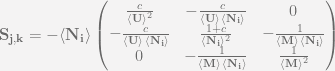
We define the vector of fluctuations in the extensive parameters as

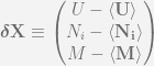
$\boldsymbol{\delta}\mathbf{X}\equiv\begin{pmatrix} U-\langle \mathbf{U}\rangle\\ N_i-\langle \mathbf{N_i}\rangle\\ M-\langle \mathbf{M}\rangle\\ \end{pmatrix}$

Rewriting the approximate macroscopic distribution function we see

$W\simeq A\; \mathrm{exp}\left[\frac{1}{2}{\boldsymbol{\delta}\mathbf{X}}^T\mathbf{S_{j,k}}\boldsymbol{\delta}\mathbf{X}\right]$

Where $\mathbf{S_{j,k}}=-\boldsymbol{\Sigma}^{-1}$ of a multivariate normal distribution. and for an ideal commodity $|\boldsymbol{\Sigma}|$ exists only for $M=M_0$ . In this case, $|\boldsymbol{\Sigma}|=\frac{\langle \mathbf{U}\rangle^2}{c}$ . When comparing data points of a time series, which is more often the case the reference state around which the values fluctuate becomes a integrated moving average, with the time dependent portion of the change in entropy represented by an AR model if it is separable. The full derivation of this point requires further work and is necessary before meaningful interpretation of actual data can be done. The interesting point here is that the equation of state simply defines a covariance matrix of a multivariate normal distribution. The more accurately we can describe a covariance matrix the better the model we can describe. Also even without knowledge of the equation of state we can make reasonable predictions, as we have in the past with conventional statistical methods. In this representation we loose the ability to gain insights provided by manipulating even a somewhat accurate equation of state.

From this perspective we can interpret the work of Ayers and Warr (2009) as providing the value obtained by bringing the commodity into the market, and then use the supply curve of energy to estimate the cost of bringing it into the market. The problem with the methodology of a conventional production function is that it treats the system as being isentropic over time. This can lead to a great deal of inaccuracies and is not a valid assumption. Ayers and Warr correct this by adapting the Cobb Douglas production function with an exponential term that somewhat approximates the relationship that we see in the utility representation of (2).

Conclusion

More work is needed in this area to estimate the performance of the macro economy. We see that the thermodynamic approach integrates well with existing econometric work and even provides a justification for the Black-Schoels model that does not explicitly make the efficient market assumption. It implies that the efficient market is the one that maximizes the entropy of the economy. It is only by looking at macro economics from the lens of statistical economics that the simple elegance and inherent complexity of the market is revealed.

We even see mathematical justification of an assertion of Adam Smith in the Theory of Moral Sentiments in the parable of the poor man’s son, where the utility obtained by procuring a good is less than the utility of the labor expended in obtaining it. Laplace described probability as common sense reduced to calculation. Thermodynamics is simply a sophisticated statistical analysis tool and when applied to economics formally shows the common sense of classical economic theory.

Bibliography

Ayres, R. U., & Warr, B. (2009). The economic growth engine: How energy and work drive material prosperity. Edward Elgar Publishing.
Card, D., & Krueger, A. B. (1997). Myth and measurement: The new economics of the minimum wage. Princeton University Press.
Cox, C. C. (1980). The enforcement of public price controls. The Journal of Political Economy, 887-916.
Friedman, M. (1994). Money mischief: Episodes in monetary history. Houghton Mifflin Harcourt.
Greene, R. F., & Callen, H. B. (1951). On the formalism of thermodynamic fluctuation theory. Physical Review, 83(6), 1231.
Johnson, W. R., & Browning, E. K. (1983). The distributional and efficiency effects of increasing the minimum wage: a simulation. The American Economic Review, 204-211.
Saslow, W. M. (1999). An economic analogy to thermodynamics. American Journal of Physics, 67, 1239.

Statistical Economics is licensed under a Creative Commons Attribution-ShareAlike 3.0 Unported License.
Based on a work at statisticaleconomics.org.

Statistical Economics

An experiment in economics & political philosophy

The Effect of Price in Macroeconomics

Abstract

Introduction

The Analogy

Bounding the Problem

Simplifying assumptions

Boundary conditions

The Money Supply

Building the Analogy

Constant utility process

Isentropic process

The Arbitrage Cycle

Buy low

Bring to market

Sell high

Adding action

Efficiency of the ideal arbitrage cycle

Impact of arbitrage on the currency

Role of Action

Conclusion

Bibliography

2 responses

Leave a comment Cancel reply

Abstract

Introduction

The Analogy

Bounding the Problem

Simplifying assumptions

Boundary conditions

The Money Supply

Building the Analogy

Constant utility process

Isentropic process

The Arbitrage Cycle

Buy low

Bring to market

Sell high

Adding action

Efficiency of the ideal arbitrage cycle

Impact of arbitrage on the currency

Role of Action

Conclusion

Bibliography

Share this:

2 responses

Leave a comment Cancel reply