Cal Abel
Atlanta, GA
Pre-alpha 0.1a

“…I believe, above all else, in reason–in the power of the human mind to cope with the problems of life.  Any calamity visited upon man, either by his own hand or by a more omnipotent nature, could have been avoided or at least mitigated by a measure of thought.”  –Bernard Baruch

Abstract

This paper advances the work of expected utility John von Neumann and Oskar Morgenstern by integrating it with the principles of J. Willard Gibbs in statistical mechanics.  The consequences of such work equate the expected marginal utility to physical force and shows how economics can be represented as classical field theory from physics.  Using the thermodynamic-economic analogies built by Wayne Saslow, the usefulness of formally linking economics to physics will lend even more powerful mathematical tools to the disposal of economists.

I. The Notion of Utility

In 1944, J. Von Neumann and O. Morgenstern developed an axiomatic approach to utility.(Neumann and Morgenstern 1944)  Their approach consisted of defining utility from a set of reasonable postulates:

1. The system of individual preferences is complete
2. Preference is transitive
   (Jaynes 1978) shows that transitivity is not required globally.
3. Preference is continuous
4. It is irrelevant in which order the constituents u, v of a combination are named (ibid pp 27)

They required one additional condition in addition to those listed above, “The simplest procedure is, therefore, to insist upon the alternative, perfectly well founded interpretation of probability as frequency in long runs.” (ibid pp19)  This is overly restrictive.  Cox identified that “[F]requency theory is inadequate in the sense that it fails to justify what is conceived to be a legitimate use of its own rules.”(Cox 1946)  If frequency theory was insufficient to be able to link statistical mechanics to thermodynamics, (Cox 1946), then it will be equally unqualified to link microeconomics to macroeconomics.

Probability as a functional property of  measurable space

The derivation of J. Pfanzagl in Theory of Measurement provides a more general derivation of subjective (Bayesian) probability with more general conditions of vNM.(Pfanzagl 1967)

Study this derivation and apply it here.  It is much cleaner/accurate than what I have. Also another source that uses the axioms (Dupre and Tipler 2009) use an axiomatic approach to derive Cox’s theorem. The axioms they chose are consistent with the axioms of von Neumann and Morgenstern.

Our first effort into this area is to identify the concept of probability as a functional over space with particular characteristics.  We shall strive for the weakest definition that contains the conditions of a measurable space as required by numeric, cardinal, utility. (need to elaborate on the basis of this the lack of need of global transitivity in order to define probability theory allows for ordinal utility in the individual however, when we apply this globally and represent a set of preferences over time or over a group of individuals or both, we express it as a statement of knowledge which based off of the space allows measurement, counting, and allows utility to be cardinal as a representation of our knowledge of the system) We first look at the requirement that the space be countable.  We have this with the finite occupancy of an individuals choices.  For a given bundle of options the individual can only chose a finite and countable set of options in a given time. Although their internal utility function is ordinal, their action in a finite time is cardinal.  It is this demonstrated preference of which our measure of knowledge of the individual is applicable.  We do not presume to know their utility function, just their actions that we can measure.  To this end the space of observed preference must be metrizable and where each open or closed set is also countable.  This is to say that the space is topologically complete.  We also require that our probability function act as a map from our metrizable space to the metric space of .  The space that contains these requirements is a perfectly normal space, or a space that is . The space also has a property that we shall use of being a  space, where all closed sets are separated from their compliments using countably many open sets, .

The space that we defined contains all measurable spaces as being metrizable.  The space contains a finite number of dimensions and is represented by  where .  We will define three closed  sets on , .  For the purposes of this exposition we will look only at the sets contained in .  This leaves three subsets of interest in  that contain  or : ,, and .

Jaynes provided a derivation of a functional equation with the appropriate form to be able to measure spaces,

where is an arbitrary function. (Jaynes 2003)

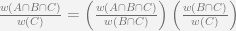
Using the definitions of the intersection of a  set with another  set is a  set and the complement of a  set being an open set .  We will define the generic  proposition space that is the complement of  as .  Using the definition of a second countable space, any subset of a second countable space is second countable, we find that, in describing the intersection of two generic spaces  and the other countable spaces resulting form  or  has the following relationship,

              (1)

We will note also that,

if and only if,           (2)

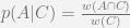
We now have enough to be able to describe the probability of a proposition space,  or , over our known information space, .  Generically, we begin defining the probability functional by looking at the proposition of  being true given that  is true.  More compactly, .  We can think of “given that  being true” as representing the known space from which we can make inference.  Another way of looking at this is that we are looking at the likelihood of  being in .  Thus our probability functional becomes:

          (3)

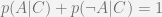
We now handily obtain the sum rule from (1) and (3):

          (4)

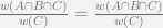
From the relationship in (2) and using (3) we obtain:

certainty is represented by           (5)

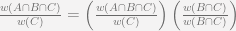
To finish the derivation of probability theory as a property of space, we will need to derive the product rule.  Using (5) we notice,

                 (6)

We then multiply the proposition again by 1 and obtain,

   (7)

Rearranging the terms we find,

             (8)

This is equivalent to,

           (9)

Using (3) and the results form (8) and (9), we obtain,

         (10)

With (4), (5), and (10) we have sufficient conditions to be able to derive the remaining necessary conditions of a complete concept of probability using the methods outlined in Chapter 2 of Jaynes’ book. (Jaynes 2003)  A careful observation will show that Bayes’ theorem (10) is property of measurable space.

Jaynes ( Jaynes 2003) basing his work on Cox and others cites three requirements for plausible reasoning.  He refers to the requirements as desiderata based on a form of weak syllogism, epagoge:

1. Degrees of plausibility are represented by real numbers.
2. Qualitative correspondence with common sense (e.g. completeness, transitivity, and continuity)
3. Reasoning is always done consistently (e.g. If a conclusion can be reasoned out in more than one way, then every possible way must lead to the same result.)

The similarity between these desiderata and vNM utility axioms is unmistakable.  The derivation of Pfanzagl (1967) shows in a formal structure that the requirement of Bayesian statistics is sufficient to meet the axioms of vNM.  What we have shown here is that in our choice of space that Bayesian statistics is a property of the space defined by von Neumann and Morgenstern’s axioms.  We shall thus only have two requirements on the condition of the space, that it is  and  measurable.  A broad definition of the allowable space for analysis, allows a much greater applicability of the theory.  We are now ready to advance with our sufficiently weak basis.

The use of a Bayesian approach allows expressing the state of knowledge of ordinal utility theory as cardinal utility, resolving the critiques against cardinal utility theory. Aczel in his refined derivation of Bayes theorem, does not rely on global transitivity. It relies only on local transitivity. To explain the significance of this, take an individual who at a certain time and with some specific quantity of information. At that moment, the individual has a transitive ordinal set of preferences for the finite set of options available to them. When this is observed over time over multiple instances, we express this knowledge of ordinal preference through the properties of countable sets in Bayesian theory. Von Neumann did this in his derivation of mixed states in quantum physics, but from a non Bayesian approach (verify his derivation).  This point will require a full proof here. The difference is in the nature of the topological space, the classical approach assumes that the space is compact, the quantum approach assumes that it is not compact.

Frequentist probability is a strong condition

We next show the frequentist approach advocated by Fisher and others as being a strong condition of our prior knowledge.  Frequentists use the definition of probability as a the frequency of an infinite number of trials.  Using the space analogy  is sufficiently large that  The other restriction is that is sufficiently large so that .  Thus the frequentist approach probability as a property of the observed phenomena vice as a representation of our state of knowledge about something.  We can see that the use of the frequentist probability theory is a special and limiting case and placing an unstated restriction on the space in which we do our analysis.

Critique of expected utility

Morgenstern (1974) while reflecting on utility stated the following:

Now the von Neumann–Morgenstern utility theory, as any theory, is also only an approximation to an undoubtedly much richer and far more complicated reality than what the theory describes in a simple manner.

From our earlier derivation, we can see that von Neumann and Morgenstern created an unnecessary restriction on utility above what they required in their axioms.  The restriction was the frequentist approach to probability theory.  This paper shall remove that restriction in a very general sense and show how to derive the macroscopic thermodynamic relationships as a property of any generic manifold.  We shall hope to provide a description of the “much richer and far more complicated reality”.  Others, particularly (Pfanzgal 1967), noted the same deficiency of vNM utility relying on an unnecessarily strong condition.

Part of the basis that Gibbs (Gibbs 1902) used to formulate statistical mechanics and then proceed to derive classical thermodynamics is the following, “It is in fact customary in the discussion of probabilities to describe anything which is imperfectly known as something taken at random from a great number of things which are completely described.” (ibid pp2)  The contrast between Gibbs’ use of probability as a representation of our state of knowledge of a system to von Neumann and Morgenstern’s use of probability as frequency in the long run is stark.  It is why this paper is being written.

We can see that how the  metric space was defined using the  axioms, satisfies the conditions of completeness, transitivity, and irrelevance of the order in which the constituents were named.  We will relax the strong requirement of the space being   to requiring the existence of an inner product, i.e.  measurable.  The most generic space that is  with a defined inner product is the Hilbert space and will be what we shall use for all future analysis.  Riemann and Euclidian space are also suitable for our purposes and only offer stronger conditions.

I need to incorporate the subjective expected utility and the critiques of Allias, and Ellsberg, and then Raffia’s comment back to Ellsworth.  This is fundamental.  It seems that the problem is not resolved because of Allias paradox, From a first glance this appears to be the result of a poorly formed problem statement based off of looking at probabilities as properties vice a representation of knowledge.  There is an element of information that is ignored.  What is the specific item that is missing?  Answer this and solve the paradox.  Another reference is Sour Grapes: studies in the subversion of rationality By Jon Elster

Resolving indifference

The Bayesian approach removes the contradiction (vNM 1944 Sect 3.3.4) where “…the individual is neither able to state which of two alternatives he prefers nor that they are equally desirable.”(ibid p19)  This is to say that each event results in a singularity for each event’s probability.  The existence of a singularity in probability violates Jaynes’ postulates.  Thus, for two events, if unable to state which of two alternatives he prefers requires that they have equal probability and represent an equivalent state of knowledge or ignorance.  Thus there is no relative preference between the two and they have the same utility.  We demonstrate this be proposing two exclusive hypotheses.  We let  represent the hypothesis ,  represent the hypothesis ,  represent the data, and  represent any prior information that we may have.  Using (10) we find,

 (11)

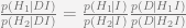
We call the term on the LHS as the “posterior” odds of .  The term on the left side of the RHS of the equation is the “prior” odds.

          (12)

We then take the natural logarithm of both sides and call  the evidence.

           (13)

We can now see that the evidence in support of one hypothesis or the other represents the difference in our uncertainty about either hypothesis.  From information theory, uncertainty is the measure of the information content of something, and is represented by:

   (14)

Table I shows the effect of the amount of change in the uncertainty between to hypotheses.  The  is exact and the odds are approximate.

Table I: Change in uncertainty between  as evidence for .

∆u	O	Prop. Strength
0	1:1	Inconclusive
1	3:1	Barely Worth Mentioning
2	7:1	Substantial
3	20:1	Strong
4	55:1	Very Strong
>4		Decisive
-∆u	1/O	Against

We can see that two hypotheses with a zero uncertainty difference represent the same probability and an equivalent amount of knowledge and are equally likely to manifest.

Axiom of Action

At this point we will have to take a detour to establish the epistemology that the theory is based on.  A survey of established literature found bits and pieces of of the necessary philosophy, but nothing that was entirely complete.  As the purpose of this paper is an outline in mathematics and economics, we will avoid a completely rigorous treatment of the epistemological underpinnings, and instead endeavor to lay out the reasoning for why what was chosen was chosen.

We do not claim to know that each actor in the economy is “rational”.  However, we will restrict our exposition of utility to those of demonstrated preference.  Thus action is required to demonstrate utility,

“Human action is purposeful behavior. Or we may say: Action is will put into operation and transformed into an agency, is aiming at ends and goals, is the ego’s meaningful response to stimuli and to the conditions of its environment, is a person’s conscious adjustment to the state of the universe that determines his life.”(Mises 1998)

We shall take this definition for the time being as it allows measurement of human behavior through observation of physical activities such as the purchase of goods or how and where time is spent.  Action in this sense describes how the individual interacts with their surroundings.  Unfortunately, von Mises’ version of action and that of others, Pierce, are philosophically insufficient for our purpose.  To quote Pierce:

This employment five times over of derivates of concipere must then have had a purpose. In point of fact it had two. One was to show that I was speaking of meaning in no other sense than that of intellectual purport. The other was to avoid all danger of being understood as attempting to explain a concept by percepts, images, schemata, or by anything but concepts. I did not, therefore, mean to say that acts, which are more strictly singular than anything, could constitute the purport, or adequate proper interpretation, of any symbol. I compared action to the finale of the symphony of thought, belief being a demicadence. Nobody conceives that the few bars at the end of a musical movement are the purpose of the movement. They may be called its upshot. But the figure obviously would not bear detailed application. I only mention it to show that the suspicion I myself expressed after a too hasty rereading of the forgotten magazine paper, that it expressed a stoic, that is, a nominalistic, materialistic, and utterly philistine state of thought, was quite mistaken.

The culmination of a series or symphony of thought as Pierce describes is the lowly and humble physical action.  He suggests in his writing that it is thought that is the culmination or symphony.  He misses the point of what a symphony is.  A symphony is series of actions of multiple individuals coordinated by the actions of a conductor, that they in themselves represent a series of actions over the span of every individuals lifetime.  They the performers have taken the time and conducted the actions necessary to be able to perform the symphony and are an ultimate expression of human will over a long period of time.  It is not important to know what they are thinking when they are playing the symphony, but that they are playing.  I contend that there is not lay person off of the street who having never laid hands on a violin, be able to take up the violin and play Beethoven’s Pastoral as one who has dedicated their life to the study of the violin and the great symphonies.

From an epistemological sense, the sum of a person’s life is the path that they have walked and the actions that they have taken along the path.  Their thoughts, not without relevance, are not necessary to judge an individuals character.  Who they are is defined by what they have done and by what they do.  We have no other metric to judge an individual.

As we saw with the derivation of (10) knowledge plays an important role in our conceptualization of the world around us.  It does not change the world, instead it changes how we interact with it.  The words that we use to describe the world, our laws that “govern” the world, are condensed expressions of our knowledge.  Their accuracy and fidelity is only a result of our knowledge.  In arbitrary space, our knowledge can apply a reasonable measure to the space we know.  It is represented by a closed set.  That which we do not know is infinite and the conjugate to our knowledge and is represented as an open set.  That is to say that it is not unknowable, but to learn we must seek to expand our knowledge.  This also shows that it is impossible to know everything.  As our knowledge becomes increasingly larger and larger it cannot express the entirety of the open set of what we do not know.

Need to address the logical independence being different form causal independence.  The actors are logically independent, that is to say that they cannot read each others minds.  This does not imply that they do not interact with each other or that their interactions are irrelevant.  The variational approach takes into account the full interactions between the actors within the manifold.

Defining utility on a manifold

The next step to take is to define the laws of microeconomic action as represented by our utility, , to cover the entire number of Hilbert spaces used to define the problem.  The Hilbert spaces are divided into two sets:  One on a manifold (intensive conditions), and the other not on the intensive manifold (extensive conditions).  The manifold need not be entirely Euclidean, but must at least be locally Euclidean.  The number of spaces on the manifold represent the degrees of freedom of the manifold.  We will describe the manifold in terms of , where each “actor”,  has  degrees of freedom.

It is important to note that the definition of what is on the manifold is completely arbitrary.  It is arbitrary to the individual who is performing the analysis as to what detail of information that they have.  More detailed the information the more of the “fine structure” is left to the space outside of the manifold.  A more succinct way of stating this is, “It depends on what you want to do.”

To proceed further we will have to make one more condition.  This condition is based on our episteme of Action.  We will adopt the requirement of stationary points of action using Hamilton’s principle.  This is a slightly different reformulation of the Euler-Lagrange stationary functional that is extensively used to describe minimum and maximum conditions, stationary condition at minima and maxima.  Hamilton’s formulation is easier for our application so we shall adopt his principle.

Hamilton’s principle:  The true evolution  of a system described in  degrees of freedom  between two specified states,  and , at two specified times,  and , is a stationary point of the action functional:

  (15)

where  is the Lagrangian function.

We will use utility to define the Hamiltonian of the system, .  The utility functional shall also be at least once differentiable and satisfy Hamilton’s formulation of the Euler Lagrange equations, meeting the “continuity condition” of vNM.  The use of a manifold allows the it to be embedded into Euclidean space using the Nash embedding theorem.  We are defining the micro economy on a manifold, so that it may be embedded into the world in which we live.  To do this, we adopt a mathematical frame work to be able to do our analysis and formally express our concepts in such a manner that we can directly apply it to application without further complications of theory.

We will define the generalized  degrees of freedom as .  We will take the reference to coordinates of the macro-economy to be in -dimensional Hilbert space.  Including time, we have a measurable space with of  dimensions.  We choose the restrictions on the space as requirements to meet the axiomatic requirements of utility.  We thus define the generic utility total derivative as:

    (16)

Since  is arbitrary will pick it to be 2, the purpose of this will become clear later on.  We will also redefine our intensive variable names, , to be , representing the intensive coordinate space, and , representing how the actors move within the manifold.  Another way of thinking of this formulation is the micro economy is entirely represented and contained by the interior of the manifold, and the macro economy is everything else.  The variable  represents time.  The ’s are coordinates to the macro-economy outside of the microeconomic manifold.

     (17)

The economic forces of the system are determined by the same generic laws of economic action.  They are a function of the coordinates microeconomic coordinates alone or in conjunction with the macroeconomic coordinates.  Thus the economic forces are a function of the ’s and ’s.  The dynamical nature of the micro-economy is a function of the ’s and ’s.

We will take an element of the manifold to be, .

Because the intensive degrees of freedom are in a manifold on a measurable space we may define the measure of  over the manifold with a density .  We can then take a the portion of the micro-economy that occupies a particular element of the symplectic manifold to be, .

Arriving at a similar point as Gibbs,(Gibbs pp8) we can extend his derivation for the total derivative of the density of states for the micro-economy to be,

For the manifold to be in statistical equilibrium the extensive forces  must be constant,

As the manifold is measurable, let the measure of the space be,

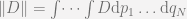
where , recalling that  is the number of degrees of freedom of the micro-economy, which is the cardinality of the space.

The probability of the phase is .  Adopting the convention of information theory, we define the uncertainty of the phase to be .  Please note the sign is different than the definition in (14).  The difference is to match the derivation of Gibbs vice following the formalism of Shannon that developed 50-years later.  This gives us,

A system in statistical equilibrium is,

, and

Gibbs formalism does not necessarily require the ergodic theory.  It is only in describing statistical equilibria that ergodicity arises.  Furthermore, systems that are in a dynamic equilibrium, that is to say systems that have not explored every possible combination of every degree of freedom but represent a set of systems that are reproducible can be handled by this theory as well.(Jaynes 1996)  As the mathematics for dynamic equilibrium are beyond the scope of what we are doing here we will limit ourselves to statistical equilibrium conditions.

II. Uncertainty Maximization (aka MAXENT)

The next step that Gibbs took was to maximize the uncertainty of the system.  He did this be selecting a set of coordinates in phase space for each degree of freedom that create a maximum uncertainty.  In our example, we will let  and  be the values of intensive momentum and position on the as yet to be defined intensive coordinate system, that give the minimum value to the uncertainty, .(Gibbs pp20) Recall here the sign is reversed from the traditional uncertainty of information theory. If the traditional notation is adopted then this becomes a maximization of .

In a non-equilibrium or dynamic equilibrium, Jaynes suggests that we use the statistical equilibrium as a maximum theoretical entropy that the system can obtain.  Thus the entropy gradient describes how far or even how fast the non-equilibrium state will drive to equilibrium or how much the system will diverge from its dynamic equilibrium state.(Jaynes 1996).

The next step in the variational approach is to expand  using a Taylor series expansion around  and .  We will only concern ourselves with the first order term, , and lump all of the higher order terms into one function, .

Recall, , which can be now rewritten as, . And we can let .  The probability of a specific element of manifold is,

We can now take the integral over the entire manifold,

Note: if the limits of each degree of freedom are ,

Recall that for a system in equilibrium,

Taking the economic forces as being conservative, (Gibbs pp 2), we can rewrite the above differential as,

We can rewrite the uncertainty as,

Because  and  are not variables that are a part of the manifold, they are extensive variables.  They are properties of the entire symplectic manifold, describing the state of the manifold in terms of the macro-economy.  They are treated as constants for the integration,

 

allowing to be determined.

We can now define the expectation of a certain function given the above relationships as,

 

A special case arises where we obtain the expected uncertainty,

 

rewritten as,

or as,

We will note the relationship of  to Shannon’s information entropy .  To avoid variable confusion we will revert to the thermodynamic notation of entropy  dropping Boltzmann’s .  The modulus of the distribution, , will be referred to as , and will contain Boltzmann’s .  This is done by, which is equivalent to saying . Where, . Thus, has the same units as utility.

Gibbs worked through the derivations of the necessary differential equations.(Gibbs pp44)  We will skip those derivations and list the key results:

Taking the last equation we will look at a system that is in equilibrium.  In order to be in equilibrium the system cannot be acted on by external forces.  Thus the forces, , are zero.  This leaves us with what we would expect to see:

and 

The equilibrium that is sought in economics between budget lines and utility functions can be thought of as following the principle of least action.  Jaynes (Jaynes 1956) identified this principle as the principle of maximum entropy.  Jaynes showed how the using a Lagrangian multiplier (least action) is the same principle as entropy maximization.  In classical demand theory the Lagrangian multiplier technique is used to resolve indifference curves with a certain budget line.  The traditional microeconomic view is that the consumer seeks to maximize their utility is fully consistent with ours.  We will note that the use of Hamilton’s principle earlier is merely an extension of entropy maximization.  The principle of maximum entropy is a part of Bayesian statistics.  By requiring Hamilton’s principle we have only admitted what we do not know and applied that within our Bayesian framework.  The only arbitrary assumption that we have is that of our ignorance.

Unstated assumption: Logical independence and freewill

Up to this point we have assumed only one thing beyond our space being  and  measurable.  We assumed logical independence of the actors within the economy.  We need to clarify between causal and logical independence.  Our actors within the economy act and interact with each other and their surroundings.  This is causal dependance.  Logical independence means they cannot read and control each other’s thoughts, that each individuals actions are independent and identically distributed.  We do not anticipate Asimov’s “Mule”.  If he were to exist, then we would have to incorporate this correlation of action, and he would be fully explained.

Some might complain that the focus on action and action alone rules out what people think and feel, that it demotes us to nothing better than dirt.  We have a few more degrees of freedom than that!  This is an important point and demands attention.  Our theory is based on the requirement of reproducible events.  We added this requirement with action.  The economy, at least the economy that we care about, is made up of reproducible events.  I can state that at least about once a week I will fill my car up with gas.  Companies make vast profit off of this reproducible event.  This is why action is so important.  Action taken that is not reproducible becomes random noise.  An individual’s rationality or even sanity is not required.  Even a demented insane person has to eat and drink or they die.  We just have much less certainty about their actions.  Stated another way, such an individual has a higher entropy than your “average Joe”.  If one has measurable behavioral characteristics that can be quantified in some form, we can take those off of the manifold and make them extensive properties.  We represent what we know and do not know through maximum entropy and the canonical distribution.  We have not left anything out.  Nor have we presumed anything that we did not originally know.  We just make better predictions based off of better information.

It is at this point that the derivations fully support the work of Saslow and integrates completely with the analogies that they built from macroeconomics to thermodynamics.  It also shows the error in the work of Smith and Foley (2005) attributing utility to entropy. Entropy is a measure of information not of utility. System representations can be done either in utility or in entropy without loss of information. This however does not make them equivalent functional relationships, which was the fundamental error of Smith and Foley. Taken together Saslow’s work and this paper provide a comprehensive framework for economic theory.  They do this without formally stating what the laws of economic action are.  Further exposition of action will be required and done in section IV.  On the Principle of Action.  For the time being we shall concern ourselves with developing marginal utility.

III. Marginal Utility

One can see that the forces acting on the system have a historic economic meaning.  For a traditional good where we let  be , some quantity of goods, we have the relationship of marginal utility as an extensive quantity and is what is measured by econometrics.

In thermodynamics,  is considered the chemical potential of the th type of particle.  Using the same analogy, and duplicate mathematical operations we will consider the marginal utility to be the economic potential of the th commodity. And represent the expected marginal utility as economic potential, .  As for the marginal utility of money we treat the money supply as a measure of the size of the system, in a similar analogy to how we treat volume in physical systems and define The total differential of a system’s expected utility then becomes,

and is composed entirely of extensive variables.  That is to say the expected utility is a canonical average of all possible combinations of every degree of freedom of the canonical assembly.  Thus traditional macroeconomic theory where each microstate was directly aggregated into the macrostate and does not include the temperature and entropy of the system will fail to accurately predict macroeconomic behavior.

To show the assumptions made in traditional microeconomics we will let the process be isentropic and consider all other economic forces other than marginal utility to be negligible.  If done that will reduce the expected utility total differential to what is traditionally seen,

The difficulty arises in that if a process occurs that is isentropic that it will often not be isothermal.  So a change in the concentrations of the products can effect the temperature of the economy.  If for example we take the change in products to be isothermal, constant level of economic activity, then to maintain a constant utility there is an additional term that arrises and is due to the aggregation of the microstates.

It is the above equation that has prevented utility from being aggregated to the macro-economy.

IV. On the Principle of Action

A careful reader will note how the development of the theory of statistical economics parallels the work of Gibbs up through and including Chapter 4 of “Elementary Principles of Statistical Mechanics”.  It is not until Chapter 5 where the laws of action are needed to further make the analogy.  If a person for whatever reason does not wish to agree with the treatment of action, they may safely stop reading and use the generic derivation of statistical economics.

Up to this point the definition of utility has been as a generic function on Hilbert space that is both differentiable and integrable (continuous and measurable).  We left the laws of economic action as being entirely undefined.  This was done to show how even with unknown laws of action that the entirety of the manifold has extensive properties, , , and  whose quantities are determined by the microeconomic laws of action.

All action in the world from the subatomic to the galactic is explained with a fair degree of accuracy by Newton’s laws of motion.  These classical laws are easily modified to incorporate relativistic effects, which explains the physical world in great detail.  Our economy relies on the transportation of goods over great distances.  It relies on the exchange of services between individuals.  The economy takes in and converts materials from the physical world then moves the finished product within the physical world, uses the products in the physical world and disposes of the products in the physical world.  Action is governed by physical laws, and as such must obey the requirements that we have previously discussed.  This is a very important observation.  Although our minds occupy the same physical world as our goods and commodities and restricted to the same laws of physics as everything else, we do not presume to be able to adequately quantify the number of degrees of freedom for the human brain.  Regardless of what one thinks, we are restricted by time, space, and energy with what we can do.  It is from this real world requirement that demonstrated preference must obey the laws of motion.  We will only concern ourselves with the classical laws of motion using Hamilton’s mechanics. OK this is the part where we get into the uncertainty principle, where there is a minimum covariance of the intensive variables, more generically the q and its simplectic form p. I need to show that this represents a minimum theoretical entropy that is an analogue to the derived form of the uncertainty principle. Thus there is some measure of minimum action. Or another way of stating this is there is a minimum temperature greater than absolute zero. I need to rework this section.

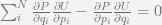
We will note three conditions of orthogonality for physical action in the micro-state:

A useful consequence of the Euler-Lagrange restriction that we applied to utility in our exposition of utility is that the Hamiltonian adopts the same functional form. (Rabei 2004)  The  we previously called economic momentum changes to become the physical momentum of the object or agent.  The only item that changed with the adoption of the physical constraint of the economy is that the economic momentum is now defined as the physical momentum of the object or agent.

The Hamiltonian listed above is for a system where all forces are conservative.  This is contradictory to our knowledge of the real world.  It is a simplification of the physics to make the mathematics easier.

In thermodynamics, a system where all forces are conservative is a system that is reversible (a.k.a. a process that is path independent).  Any introduction of non-conservative forces adds irreversibility.  F. Riewe (Riewe 1995) developed a Hamiltonian that takes into account frictional forces.  Riewe’s approach was further refined by E. Rabei et al. (Rabei 2004)

The discussion of irreversibility of the system is important to address.  It requires that energy continually be added in order to keep objects in motion.  Think of this as filling up a tank of gas in a tractor-trailer that is transporting goods.  Without the addition of the useful work from combusting the diesel fuel, the goods would not go anywhere.

With utility now on a stronger theoretical footing, we can work toward further developing the theory.  Recall, utility is restricted to demonstrated preference.  For the time being, we will be concerned only about physical goods and services.  We will later turn to information goods and services. These topics will be the subject of future papers.

Bibliography

• Ayers, R. U. and B. Warr (2009). The Economic Growth Engine: How Energy and Work Drive Material Prosperity. Northhampton, MA, International Institute for Applied Systems Analysis.
• Axelrod, R. and W. D. Hamilton (1981). “The Evolution of Cooperation.” Science 211(4489): 1390-1396.
• Callen, H. B. (1985). Thermodynamics and an Introduction to Thermostatistics. New York, John Wiley & Sons.
• Cox, R. T. (1946). “Probability, Frequency and Reasonable Expectation.” American Journal of Physics 14(1): 1-13.
• Dupré, M. J. and F. J. Tipler (2009). “New axioms for rigorous bayesian probability.” Bayesian Analysis 4(3): 599-606.
• Gibbs, J. W. (1902). Elementary Principles in Statistical Mechanics Developed with Especial Reference to The Rational Foundation of Thermodynamics. New York, Charles Scribner’s Sons.
• Greene, R. F. and H. B. Callen (1951). “On the formalism of thermodynamic fluctuation theory.” Physical Review 83(6): 1231.
• Jaynes, E. T. (1957). “Information Theory and Statistical Mechanics.” Physical Review 106(4): 620-630.
• Jaynes, E. T., Ed. (1983). Where Do We Stand on Maximum Entropy? E. T. Jaynes: Papers on Probability, Statistics and Statistical Physics. Dordrecht NL, Kluwer Academic Publishers.
• Jaynes, E. T. (1985). “Macroscopic Prediction.” Complex Systems – Operational Approaches.
• Jaynes, E. T. (1986). Predictive Statistical Mechanics. Frontiers of Nonequilibrium Statistical Physics. G. T. Moore and M. O. Scully. New York, Plenum: 33-55.
• Jaynes, E. T. (1991). The Second Law As Physical Fact and As Human Inference. St. Louis, MO, Washington University: 10.
• Jaynes, E. T. (1991). “How should we use entropy in economics?”.
• Jaynes, E. T. (2003). Probability Theory: The Logic of Science, Cambridge University Press.
• Luzzi, R., A. R. Vasconcellos, et al. (2002). Predictive Statistical Mechanics. Dordrecht, Kluwer Academic Publishers.
• Mas-Colell, A., M. D. Whinston, et al. (1995). Microeconomic Theory. New York, Oxford University Press.
• Mises, L. v. (1998). Human Action: A Treatise on Economics. Auburn, Ludwig von Mises Institute.
• Morgenstern, O. (1974). Some Reflections on Utility, New York University Press.
• Neumann, J. v. and O. Morgenstern (1944). Theory of Games and Economic Behavior, Princeton University Press.
• Neumann, J. v. (1955). Mathematical Foundations of Quantum Mechanics. Princeton, Princeton University Press.
• Pfanzagl, J. (1967). Subjective Probability Derived from the Morgenstern-von Neumann Utility Concept. Essays in Mathematical Economics. M. Shubik. Princeton, NJ, Princeton University Press: 237-251.
• Rabei, E. M., T. S. Alhalholy, et al. (2004). “On Hamiltonian Formulation of Non-Conservative Systems.” Turkish Journal of Physics 28: 213-221.
• Saslow, W. M. (1999). “An Economic Analogy to Thermodynamics.” American Journal of Physics 67(12): 1239-1247.
• Shannon, C. E. (1948). “A Mathematical Theory of Communication.” The Bell System Technical Journal 27: 379-423, 623-656.
• Smith, E. and D. K. Foley (2005). “Classical thermodynamics and economic general equilibrium theory.” Journal of Economic Dynamics and Control 32(1): 7-65.
• Van Horn, K. S. (2003). “Constructing a logic of plausible inference: a guide to Cox’s theorem.” International Journal of Approximate Reasoning 34(1): 3-24.

 

Statistical Economics is licensed under a Creative Commons Attribution-ShareAlike 3.0 Unported License.
Based on a work at statisticaleconomics.org.